Estimating Regime Switching Models For Electricity Prices
November 2025 (3215 Words, 18 Minutes)
I would like to start by giving you a little bit of context and the foundations of this article.
I’m writing it while working on a broader topic: computing Cash-Flows at Risk for a gas-fired power plant. I’ve defined a simple workflow to guide the modelling process:
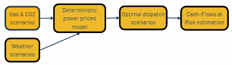
I’ve already shared a Linkedin post about the co-simulation of gas and CO2 scenarios. I’m now focusing on generating power prices based on fundamental variables such as gas and CO2 prices and weather. My first idea was to use an Machine Learning model to derive prices from these inputs. Thanks to the scenarios I’ve created to simulate the level of these inputs for future periods, I’ll be able to feed my model and have a range of power prices. My concern is that standard Machine Learning models often struggle to capture extreme events which are quite frequent on power markets.
In a previous article, I described how we can model jumps using a Poisson process, but I decided not to use the same method here (it wouldn’t have been fun). That’s why I’ve chosen a different approach called Regime Switching (RS). The intuitiveidea behind RS is the existence of different states of the market (for example: a “crisis state” vs a “normal state”), and the fact that the market switches from one state to another following a Markov chain.
You’ll notice that the section about the estimation of the Hidden Markov Model behind the regime switching approach is more technical than the rest of the article. I found this section important because it explains how a complex problem like the one we’ll go through can be managed by applying the correct optimisation methods. However, skipping this section will not hurt your ability to understand the overall message of this article.
Now that the context is set, let’s dive into the process of setting up a regime switching model for power prices. I’ll come back at the end of the article on how I will use it for my purpose.
1. Managing the seasonality
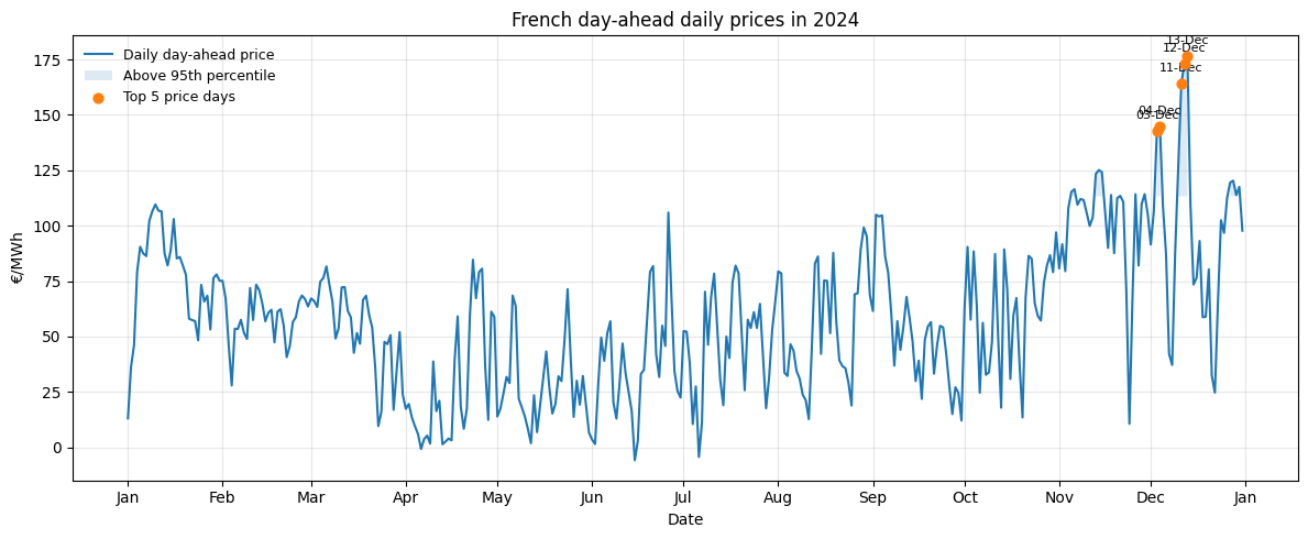
We work with daily power prices, obtained by averaging hourly (or quarter-hourly) observations over each day. In this article, I use French day-ahead prices from January 2023 to October 2025.
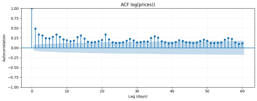
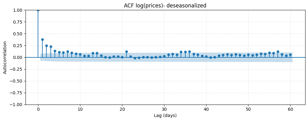
The seasonality of power prices has been well documented and can be observed in our dataset through the autocorrelation plot below which shows pronounced peaks at multiples of 7 (a signature of a weekly pattern).
To estimate our regime-switching model, we want to remove this seasonality and work with a deseasonalised series. Following a classical decomposition, we express the (log) spot price as:
\[\log(\text{Price}_t) = S_t + X_t\]where
- \(S_t\) is a deterministic seasonal component, and
- \(X_t\) is a stochastic component (the part we will model with the regime-switching process).
Using log-prices stabilizes variance, making the stochastic component \(X_t\) closer to Gaussian and easier to model with regime switching.
We do not want \(S_t\) to include any fundamental variable, it should only represent the calendarian evolution of the power price. That’s why we can modelize it like :
\[S_t = \sum_{d=1}^{7} a_d \cdot \text{DOW}_{t,d} \;+\; \sum_{m=1}^{12} b_m \cdot \text{Month}_{t,m}\]where \(DOW\) means day of the week. You can see that it’s just a regression on two calendar dummy variables (day of the week and month).
I’ve also tested trigonometric seasonality but it tends to smooth transitions, whereas electricity markets exhibit sharp discontinuities between weekdays and weekends. Dummy variables capture these discontinuities better.
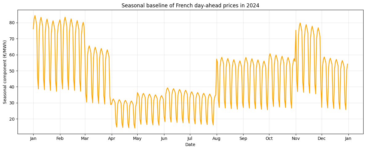
When plotting \(S_t\), we clearly observe seasonal patterns consistent with the weekly and annual cycles (decrease in price during week-ends and summer).
Subtracting this seasonal component to the log-prices gives us the deseasonalised series \(X_t\). The ACF of \(X_t\) shows that most of the seasonality has been removed :
On the chart below, the left panel shows the distribution of raw log-prices, which is heavily skewed because of strong weekly and yearly seasonal patterns. After removing seasonality, the right panel shows a much more symmetric and centred distribution, with extreme values now clearly identifiable as genuine market shocks rather than calendar effects.
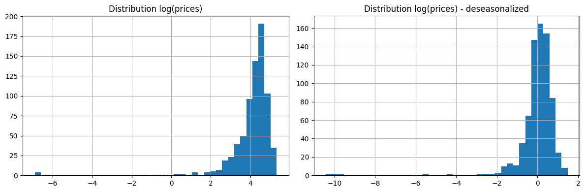
This deseasonalised series is therefore a more suitable input for estimating regime-switching dynamics.
2. Understanding how the Regime-Switching model works
As discussed in the introduction, the intuition behind Regime Switching is that we cannot model the behaviour of power prices using a single stochastic process. The dynamics of prices depend strongly on the state of the system. For example, we may assume that volatility increases when the system enters a “crisis” mode.
For this reason, we define a small number of distinct regimes (in this article, we will compare a 2-regime setup to a 3-regime setup). Each regime has its own mean, volatility, and short-term dynamics — all wrapped inside an AR(1) model.
🧠 A Note on AR(1) models
An AR(1) model (“Auto-Regressive model of order 1”) is one of the simplest ways to describe how a variable depends on its own past values. In an AR(1) process, today’s value is a combination of:
- A long-term mean
- A fraction of yesterday’s deviation from that mean
- Random noise
Mathematically we can write :
\[X_t = \mu + \phi (X_{t-1} - \mu) + \sigma \varepsilon_t, \qquad \varepsilon_t \sim \mathcal{N}(0,1)\]It can be read as :
-
If \(\mid \phi \mid < 1\), the process pulls back toward its mean \(\mu\) over time → this is mean reversion.
-
If \(\phi = 0\), there is no memory (pure noise).
-
If \(\phi\) is close to 1, the process keeps memory of past shocks → effects of shocks are persistent.
-
The parameter \(\sigma\) controls the volatility of the innovations.
AR(1) makes the model simple, interpretable, and easy to estimate, while capturing the essentials of electricity-price dynamics.
Now that we have defined how the price will behave within each state, we need to explain how it goes from one state to another.
2.1 Using an Hidden Markov Model
Let’s remember first what are the Markov property and Markov chains:
🧠 A Note on Markov chains
A stochastic process \((S_t)\) is said to satisfy the Markov property if the future depends only on the present state, not on the past. Formally:
\[\mathbb{P}(S_{t+1} = j \mid S_t = i, S_{t-1}, S_{t-2}, \ldots ) = \mathbb{P}(S_{t+1} = j \mid S_t = i).\]In words:
“Knowing where you are is enough to know where you are going next.”
This property allows us to summarize the entire dynamics using a transition matrix containing the probabilities of switching from one state to another.
We start with an example of a “not-hidden” markov chain. Suppose we categorize weather into three observable states:
- 1 = Sunny
- 2 = Cloudy
- 3 = Rainy
If we have 5 years of daily weather data, we can count transitions such as:
- how often “Sunny” is followed by “Sunny”
- how often “Sunny” is followed by “Cloudy”
- how often “Cloudy” is followed by “Rainy”
- etc.
Dividing the counts by row totals gives the empirical transition matrix \(P\) with in line the current state (from top to bottom : Sunny, Cloudy, Rainy) and in colums the future state (from left to right : Sunny, Cloudy, Rainy). Each value represents to probability to go to the future state (column) knowing the current state (line):
\[P = \begin{pmatrix} 0.70 & 0.20 & 0.10 \\ 0.30 & 0.50 & 0.20 \\ 0.15 & 0.25 & 0.60 \end{pmatrix}\]Here:
- a Sunny day is followed by another Sunny day 70% of the time
- a Rainy day becomes Cloudy the next day 25% of the time
- etc.
Because states are directly observed, inference is straightforward.
But in many financial and energy applications (including ours), the true state of the system (e.g., “normal”, “stress”) is not observed : we only see the resulting prices.
This leads us to a Hidden Markov Model (HMM), where the states are latent but the prices provide noisy information about which state we are likely in.
To summarize, building a regime-switching model means estimating many things at once:
- the behaviour of prices inside each regime (mean, mean reversion, volatility),
- the probabilities of jumping from one regime to another,
- and the hidden sequence of regimes over time.
Because none of these quantities are directly observable, the model must infer them simultaneously. This creates a highly interdependent and time-consuming estimation problem:
→ changing the dynamics inside one regime modifies the most likely regime sequence,
→ which then modifies the transition probabilities,
→ which then modifies the likelihood of all parameters… and so on.
This is why we rely on numerical optimisation and algorithms like Hamilton’s filter : the following section describes that (and can be skipped if you prefer → go Here).
3. Estimating the Regime-Switching model
3.1 Maximizing the likelihood
To estimate our regime-switching model, we need a way to measure how well a set of parameters explains the observed price series. This is exactly what the likelihood does.
Likelihood = given my parameters, how probable is it that I observe this data?
If the model assigns high probability to the prices we actually observed, the parameters are good. If the model says these prices were very unlikely, the parameters are bad.
Because multiplying thousands of probabilities quickly leads to tiny numbers, we work instead with the log-likelihood, which turns products into sums and is much easier to optimise numerically.
In a regime-switching (Hidden Markov) model, the log-likelihood combines:
- the probability of being in each hidden regime at each date,
- the probability of observing the price given the regime’s AR(1) dynamics,
- the probability of switching from one regime to another according to the transition matrix.
Formally, let:
- \(x_t\) be the observed (deseasonalised) log-price,
- \(s_t \in \{1,\dots,K\}\) the hidden regime at time \(t\),
- \(f(x_t \mid s_t, \theta)\) the AR(1) density in regime \(s_t\),
- \(P_{ij} = \mathbb{P}(s_t = j \mid s_{t-1} = i)\) the transition matrix.
- \(\pi_{s_1}\) is the initial probability distribution over the regimes
For a given sequence of hidden states \(s_1,\dots,s_T\), the likelihood is:
\[L(x_{1:T}, s_{1:T} \mid \theta) = \pi_{s_1}\, f(x_1 \mid s_1) \prod_{t=2}^{T} P_{s_{t-1}, s_t} \, f(x_t \mid s_t),\]and the log-likelihood is:
\[\ell = \log \pi_{s_1} + \log f(x_1 \mid s_1) + \sum_{t=2}^{T} \big( \log P_{s_{t-1}, s_t} + \log f(x_t \mid s_t) \big).\]But we do not observe the true states \(s_t\). Therefore the log-likelihood of the HMM is the weighted sum over all possible state paths:
\[\ell(\theta) = \log \sum_{s_{1:T}} L(x_{1:T}, s_{1:T} \mid \theta),\]which will require a specific method, such as the Hamilton filter, to be computed efficiently.
The goal of estimation is simple: find the parameters \(\theta\) that maximise the log-likelihood, i.e. the parameters under which the observed prices are the most “expected” by the model.
3.2 The Hamilton Filter: estimating hidden regimes
Since we do not know which regime generated each observation, we cannot simply count transitions or estimate AR(1) parameters per regime. The Hamilton filter (Hamilton, 1989) provides a recursive way to infer, at every date, the probabilities :
\[P(s_t = j \mid x_{1:t})\]updating uncertainty as new prices arrive through the Markov transitions and Bayes’ rule. It lets us track the hidden regimes in real time and compute the likelihood needed for optimisation.
3.2.1 Hamilton Filter Algorithm with example
Assume:
- 2 regimes,
- transition matrix (values are manually chosen here)
- regime-specific AR(1) densities \(f_1(x_t)\) and \(f_2(x_t)\).
We denote:
- \(\alpha_{t\mid t} = P(s_t \mid x_{1:t})\) = filtered probability,
- \(\alpha_{t\mid t-1} = P(s_t \mid x_{1:t-1})\) = predicted probability.
Step 1️⃣ — Initialise regime probabilities
What the algorithm does:
We pick a starting distribution for the regimes before observing any data.
Example:
We start with no reason to believe the system is more likely in either regime (well, in practice, that’s generally not true).
Step 2️⃣ — Prediction step (Markov propagation)
What the algorithm does:
We use the transition matrix to predict the probability of being in each regime before seeing today’s price.
The formula is:
\[\alpha_{t|t-1}(j) = \sum_{i=1}^2 \alpha_{t-1|t-1}(i)\, P_{ij}.\]Example: (predicting today’s regimes from yesterday’s beliefs):
Suppose yesterday we had:
Then:
\[\alpha_{t|t-1}(1) = 0.7 \cdot 0.9 + 0.3 \cdot 0.2 = 0.69,\] \[\alpha_{t|t-1}(2) = 0.7 \cdot 0.1 + 0.3 \cdot 0.8 = 0.31.\]We now have predicted probabilities before observing today’s price.
Step 3️⃣ — Filtering step (Bayesian update with today’s price)
What the algorithm does:
We update the predicted probabilities using how likely today’s price is under each regime.
Update formula:
\[\alpha_{t|t}(j) = \frac{ f_j(x_t)\, \alpha_{t|t-1}(j) }{ \sum_{k=1}^2 f_k(x_t)\, \alpha_{t|t-1}(k) }.\]Example:
Suppose today’s price is unusually high. The regime-specific densities evaluate to:
Weighted likelihoods:
\(\tilde{\alpha}_1 = 0.01 \times 0.69 = 0.0069,\) \(\tilde{\alpha}_2 = 0.20 \times 0.31 = 0.062.\)
Normalisation:
\[\alpha_{t|t} = \left( \frac{0.0069}{0.0689},\; \frac{0.062}{0.0689} \right) = (0.10,\; 0.90).\]After observing the spike, regime 2 becomes far more likely.
Step 4️⃣ — Update the log-likelihood contribution
What the algorithm does:
We compute today’s contribution to the log-likelihood so the optimiser can later find the best parameters.
Contribution:
\[L_t = \sum_{j=1}^2 f_j(x_t)\, \alpha_{t|t-1}(j).\]The total log-likelihood is:
\[\log \mathcal{L} = \sum_{t=1}^T \log L_t.\]Example:
\[L_t = 0.0069 + 0.062 = 0.0689, \qquad \log L_t = -2.6768.\]This value is added to the total log-likelihood, which the optimiser later tries to maximise.
3.2.2 Summary
At each date, the filter:
- Predicts regime probabilities using the Markov chain.
- Updates them using today’s price and Bayes’ rule.
- Adds the contribution to the log-likelihood.
This recursion makes the Hidden Markov Model estimable even though the regimes are never observed directly.
3.3 Parameter estimation: maximisation procedure and smoothing
Once we know how to compute the log-likelihood of the model using the Hamilton filter, the next step is simply to find its maximum:
\[\widehat{\theta} = \arg\max_{\theta} \log \mathcal{L}(\theta),\]where \(\theta\) groups all already discussed parameters.
Because the log-likelihood is not linear and has no closed-form solution, we must rely on numerical optimisation.
The idea is :
- Choose a trial parameter vector \(\theta\).
- Run the Hamilton filter to compute the log-likelihood.
- Change \(\theta\) slightly (via an optimisation algorithm).
- Keep the version that gives a higher log-likelihood.
- Repeat until improvements become negligible.
Even though the internal math is complicated, the procedure is always the same: the optimiser tries different parameter values until it finds the ones that make the observed prices most “expected” under the model.
4. Results
This section presents the main outputs of the regime-switching modelling applied to the deseasonalised daily day-ahead power prices. It also describes an alternative to Regime Switching with constant transition probabilities (check here)
4.1 Model Comparison and Selection
The 3-regime Markov Switching model (MRS-3) achieves by far the highest log-likelihood (–288.3) than the 2-regime model (-675), indicating a substantially better fit to the data.
This aligns with empirical intuition: power prices exhibit three distinct statistical behaviours—normal, stressed-low, and stressed-high—that cannot be captured using only two regimes.
I also tried two alternatives to the specifications discussed in this article:
- a definition of states based on fixed thresholds (e.g., days where anomalies fall below or above a certain percentile such as the 5th or 95th),
- a time-varying transition probability model (described at the end of this section), which allows transition probabilities to depend on market conditions such as gas prices, month of the year, or residual load.
The first option was a bit too simple but can really help for the initialisation of the optimisation. The second, apparently promising, didn’t give good results in my case (I’ll need to work on it).
4.2 Regime Classification Over Time
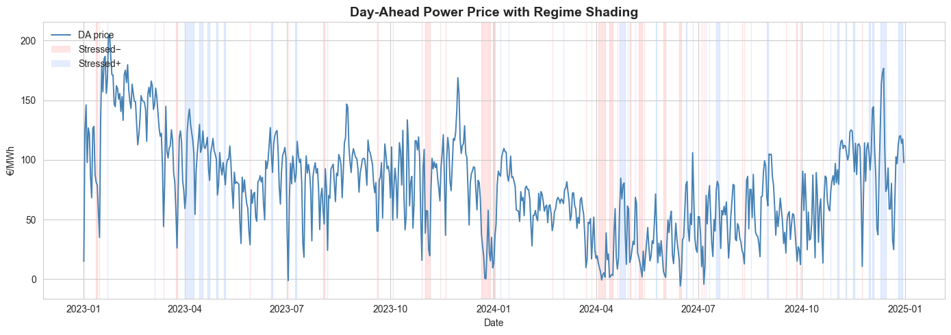
The figure below shows the observed daily day-ahead prices over 2023–2024, with background shading highlighting the inferred regimes of the 3-state Markov Switching model:
- Stressed− (red bands) → exceptionally low anomalies
- Normal (unshaded) → central behaviour
- Stressed+ (blue bands) → exceptionally high anomalies
Periods of market stress coincide with large deviations in the daily prices, often associated with weather shocks, demand surges, or supply constraints.
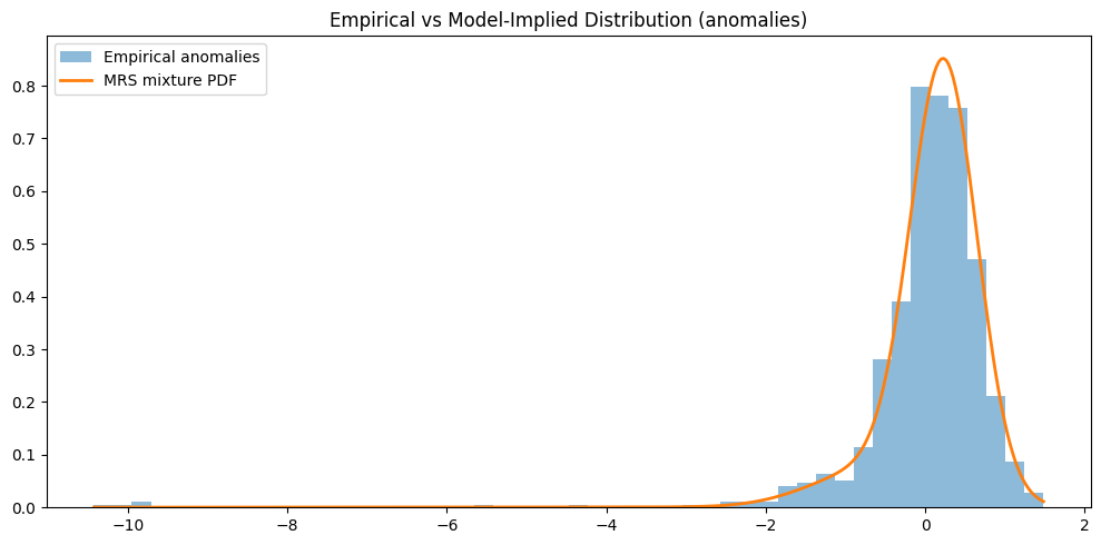
4.3 Fit to the Empirical Distribution
To evaluate how well the model reproduces the statistical properties of daily price anomalies, we compare:
- the empirical distribution of deseasonalised log-price anomalies (histogram), and
- the model-implied mixture distribution obtained by combining the three Gaussian AR(1) regimes using their stationary regime probabilities.
The match is good, especially around the centre of the distribution. The model captures moderate volatility clustering and asymmetric behaviour, though the tail events remain difficult to fully represent with Gaussian components alone—this is a known challenge in electricity markets.
4.4 Transition Matrix and Key Takeaways
The transition matrix is maybe the most important result for what I want to do then :
\[P = \begin{pmatrix} 0.49 & 0.50 & 0.00 \\ 0.06 & 0.88 & 0.05 \\ 0.01 & 0.43 & 0.56 \end{pmatrix}\]This transition matrix shows that the “normal” regime (middle row) is highly persistent (88% chance of staying) and acts as a hub, since both stressed regimes frequently move back into it. The stressed regimes are short-lived (only 49% and 56% persistence) and highly asymmetric: stressed– almost always returns to normal, while stressed+ sometimes jumps directly down into stressed–.
To summarise this section :
- A 3-regime structure provides the most realistic representation of observed price dynamics.
- The model’s mixture density reproduces the central part of the empirical distribution well.
- Regime classification over time reveals meaningful clusters of stressed price behaviour.
- These results justify using the 3-regime model as the basis for scenario generation, jump modelling, and probabilistic forecasting.
🧠 A Note on Time-Varying Regime Switching
In the standard Markov Regime Switching (MRS) model, transitions between regimes are governed by a constant probability matrix.
This assumes that the likelihood of moving from one state to another never changes. But in electricity markets, regime changes often depend on observable fundamentals such as gas prices, residual load, seasonality, or weather conditions.
The Time-Varying Regime Switching (TVRS) model generalises MRS by making transition probabilities depend on a vector of explanatory variables denoted by \(z_t\).
In this case, transitions become:
\[P(s_t = j \mid s_{t-1} = i, z_t) = P_{ij}(z_t).\]To ensure that each row still sums to one, a multinomial logit specification is used. For each departure regime \(i\):
\[P_{ij}(z_t) = \frac{\exp(\beta_{ij}^T z_t)} {\sum_{k=1}^{K} \exp(\beta_{ik}^T z_t)}.\]Here, \(\beta_{ij}\) is a vector of coefficients that describes how the variables in \(z_t\) influence the transition from regime \(i\) to regime \(j\).
Inside each regime, the price anomalies can still follow a regime-specific AR(1) process:
\[X_t = \mu_s + \phi_s (X_{t-1} - \mu_s) + \sigma_s \varepsilon_t, \qquad \varepsilon_t \sim \mathcal{N}(0,1).\]The key idea is that regime changes are no longer purely random: they become conditional on market conditions. When fundamentals signal tension (for example high residual load or high gas price), the probability of entering a stressed regime increases. When fundamentals normalise, the model naturally shifts probability back toward calmer regimes.
5. The next Step
In the introduction, I explained that my objective is to combine a regime-switching model with an hourly Machine Learning model to generate power price scenarios that are both realistic on average and capable of reproducing extreme events.
As of today (November 27th, 2025), I am still evaluating two different integration strategies. Very soon, you will be able to see which one I selected, why and how this hybrid approach can be used to simulate hourly price paths that incorporate both fundamental drivers and regime-dependent volatility.
Reference sources
- Hamilton (1989), New approach to economic time series with regime switching
- Lucia, Schwarz (2000), Electricity prices and power derivatives. - Evidence from the Nordic Power Exchange
- Perlin (2015), HMM in Finance