Simulating Electricity Spot Prices With Jump Diffusion Model
September 2025 (2017 Words, 12 Minutes)
Electricity spot prices don’t behave like other commodities or financial assets — they have their own personality, and it’s a bit wild. The main reason is the non-storability of electricity: supply and demand must be balanced every second. Any imbalance between consumption and generation can push prices sharply up or down.
There is some good news, though: price patterns are highly predictable in shape because seasonality is everywhere:
- During a day, we usually see morning and evening peaks surrounding the midday solar dip.
- During a week, consumption drops on weekends compared to weekdays as business activity slows down.
- Across the year, prices vary with the seasons: heating in winter, cooling in summer, and hydrology in spring.
So the shape of prices is quite regular. The challenge is that the magnitude of prices is much harder to predict.
In this article, we’ll focus on three other important features of electricity spot prices that we need to capture in models:
- Strong mean-reversion: Unlike stocks, power prices don’t wander off indefinitely. Deviations from normal levels tend to snap back quickly.
- Spikes and crashes: Sudden extreme highs or very low (even negative) prices. Short-lived but critical for risk.
- Negative prices (in renewables-heavy systems): Generators may pay to stay online; not every process allows negative values, which challenges modeling choices.
Because of these characteristics, plain vanilla finance models aren’t enough — we need to adapt and extend them.
Demystifying stochastic processes
Spoiler: you won’t escape stochastic processes in this article — they’ll be everywhere.
But I promise that even without a PhD in mathematics, you’ll be able to follow along easily. In the end, although the term may sound intimidating, it simply means a way to describe something that evolves randomly over time.
A stochastic process is a bit like your child: you can’t control or predict their exact next move. That’s the essence of randomness. So instead, we take a step back and define the framework within which they can evolve.
Instead of predicting the exact next step, we describe the rules of randomness that govern the journey.
In this article, we’ll use two of the most common building blocks: Brownian motion and the Poisson process.
Brownian motion
It’s a hot summer night in Paris, the atmosphere is festive because the national football team has just won the World Cup — again. Walking down the street, you recognize a friend, drunk, and stop to observe his chaotic progression. Left, right, forward, backward… over time his path looks messy. That’s essentially Brownian motion: tiny moves that, when accumulated, create an unpredictable path.
In finance, it’s been used to model stock prices: they drift and wiggle continuously, never quite moving in a straight line. We call it Brownian thanks to a Scottish botanist, Robert Brown, who in 1827 observed the erratic movement of pollen particles suspended in water.
At this point you may be thinking: “Thank you for the history lesson, but what makes this random process special enough to have its own name?” That’s where the math comes in:
- A Gaussian process is continuous: no teleportation.
- A Gaussian process has no memory: current and past positions don’t influence the next move.
- The average displacement is zero: if you simulate many Gaussian processes starting from the same point, their average position at time \(t\) will still be the starting point.
- But the spread increases over time: the more paths you simulate, the further apart the extremes will drift.
We also write, for a Brownian (also called Wiener) process \(W_t\):
\[dW_t \sim \mathcal{N}(0, dt)\]which means that in a very small time step \(dt\), the change in \(W_t\) is normally distributed with mean 0 and variance equal to the length of that time step.
Poisson process
I remember waiting at a bus stop with my friends as a kid, betting on when the next bus would arrive. Sometimes we waited a long time, sometimes two came close together — even if, on average, the number of buses per day was always about the same. Too bad I didn’t know about the Poisson process back in 2010… it might have helped me win more bets (well, not really, because as we’ll see, stochastic processes aren’t used for forecasting exact outcomes).
Mathematically, if \(N_t\) is a Poisson process with rate \(\lambda\):
\[\Pr(N_t = k) = \frac{(\lambda t)^k}{k!} e^{-\lambda t}, \quad k=0,1,2,\dots\]which means the probability of seeing \(k\) events up to time \(t\) follows a Poisson distribution.
One of its defining features is that the number of arrivals in disjoint time intervals are independent, and the average number of arrivals grows linearly with time (\(\lambda t\)).
What we are going to do (and not do)
We’ve talked about stochastic processes and electricity spot markets. Now comes a key question:
Do you think we’ll use a stochastic model to predict tomorrow’s spot price?
The answer is no. The models we’ll discuss here have a very different objective.
We want to reproduce the key features of electricity markets: the wiggles, the tendency to come back to a normal level, those occasional crazy spikes, and the possibility of negative prices. This will allow us to create a distribution of scenarios, capturing both ordinary days and extreme events.
Why is that useful? Because in power markets — and in risk management more generally — we don’t just care about the most likely outcome. We also care about:
- the risk of price spikes,
- the probability of very low or even negative prices,
- the impact of volatility on contracts, revenues or hedges.
Think of it this way:
- Forecasting is like asking “What’s the weather going to be tomorrow at 3 pm?”
- Stochastic modeling is more like “If I simulate many possible weather patterns, what does the range of outcomes look like? How likely are storms, sunshine, or heat waves?”
With a stochastic model we obtain a distribution of possible futures, not just one prediction. That’s why, in the rest of this article, we’ll walk through a series of increasingly realistic models: starting from a simple random walk, then adding mean reversion, and finally introducing jumps.
Simple Random Walk (Geometric Brownian Motion)
Let’s start slowly with a classic model called the Geometric Brownian Motion (GBM).
You’ll quickly see that this model is not sufficient for electricity prices, but it’s a useful stepping stone to understand the logic behind more complex combinations of stochastic processes.
The stochastic differential equation (SDE) is:
\[dS_t = \mu S_t \, dt + \sigma S_t \, dW_t\]- The first term, \(\mu S_t dt\), is deterministic, with \(\mu\) representing the drift rate — the average trend of prices.
- The second term, \(\sigma S_t dW_t\), is stochastic, with \(\sigma\) being the volatility (it controls how wild the swings are), and \(dW_t\) the random “wiggle” from Brownian motion.
- Both parts are multiplied by \(S_t\), which means that the higher the price, the larger the absolute moves. That’s why GBM generates percentage changes rather than fixed increments.
By solving the SDE, we get the closed-form solution:
\[S_t = S_0 \exp\Big[ \Big(\mu - \tfrac{1}{2}\sigma^2\Big)t + \sigma W_t \Big]\]From this exponential form, we immediately see one important property: prices stay strictly positive.
But that’s not really the main issue for us. Imagine you are Little Red Riding Hood, trying to cross a forest to reach your grandmother’s house. At every intersection, you flip a coin to decide which path to take. What will prevent you from drifting critically away from your destination? Nothing.
That’s exactly the problem with GBM: without any mechanism to pull prices back, the path can wander off indefinitely.
For electricity markets, that’s a dealbreaker. We need to force mean reversion; otherwise, our simulated prices will drift away, just like in the plot below:
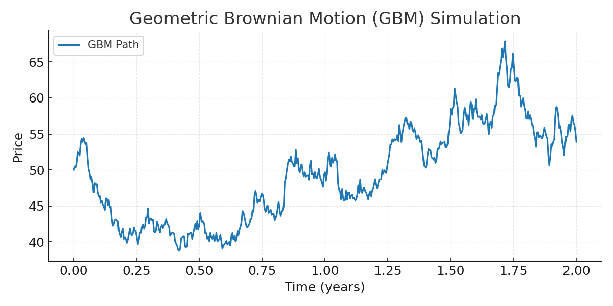
In fact, GBM is a decent model for stocks, where prices can indeed drift away without bound. But for electricity prices, it doesn’t capture mean reversion, seasonality, or spikes — all of which are essential.
Ornstein–Uhlenbeck process
To bring mean reversion into our model, we need to tweak things a little.
The Ornstein–Uhlenbeck (OU) process is written as:
\[dS_t = \alpha(\mu - S_t)\,dt + \sigma\,dW_t\]Here’s what each parameter does:
- \(\mu\) is the long-term mean level. Prices are “magnetized” toward this value.
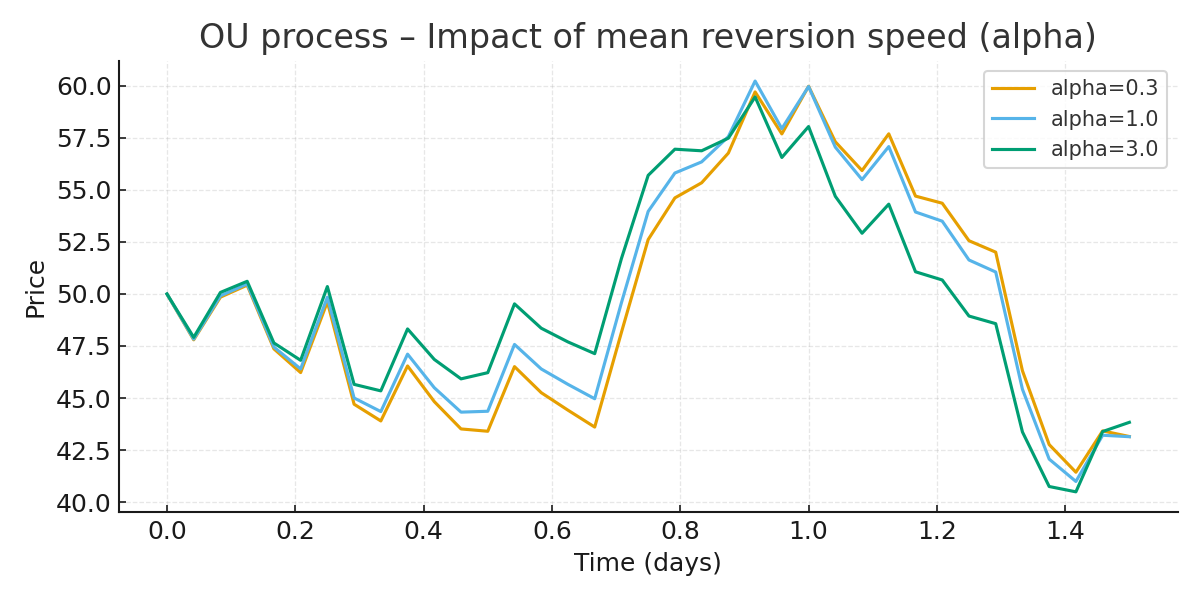
- \(\alpha\) is the speed of mean reversion. It tells us how strong the pull of the magnet is:
- A high \(\alpha\) means prices snap back quickly.
- A low \(\alpha\) means they drift around lazily before returning.
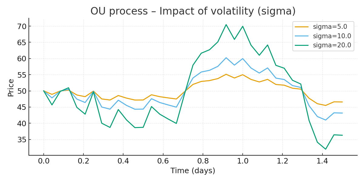
- \(\sigma\) is the volatility. The bigger it is, the more prices wiggle around on their way back to \(\mu\).
On the following plot, you can observe the impact of volatility (with \(\alpha\) = 1 and \(\mu\) = 50) :
And on this one, the speed of mean reversion varies (\(\mu\) = 50 and \(\sigma\) = 10) :
👉 Imagine a ball attached to a spring: if you pull it away from the center, the spring (mean reversion) pulls it back. The stiffness of the spring is \(\alpha\), the center point is \(\mu\), and your shaky hand bumping the table is \(\sigma\).
Below is a simulation of a OU process with \(\alpha\) = 1, \(\mu\) = 50, \(\sigma\) = 10 and \(S_0\) = 50
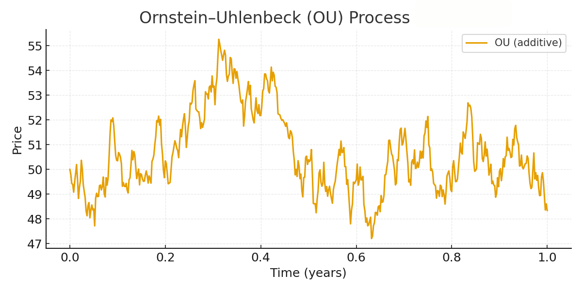
This additive version can generate negative prices, which is problematic if we want to enforce strictly positive values. That’s where the log-OU version comes in:
\[d(\ln S_t) = \alpha(\mu_L - \ln S_t)\,dt + \sigma\,dW_t\]- \(\mu_L\) is the long-term mean of the log-price.
- \(\alpha\) and \(\sigma\) play the same roles as before.
Because the dynamics happen on the log scale, the actual price is always:
\[S_t = \exp(\ln S_t) > 0\]So the log-OU is strictly positive and keeps the same mean-reverting logic. Below is a simulation of a OU process with \(\alpha\) = 1, \(\mu\) = ln(50), \(\sigma\) = 0,25 and \(S_0\) = 50
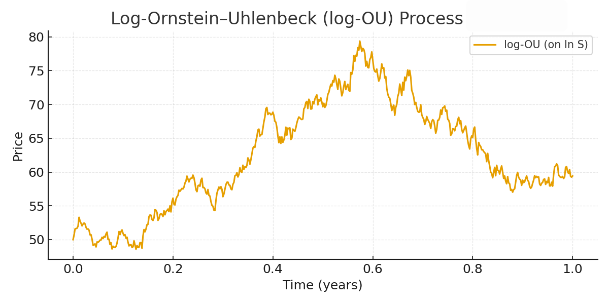
The OU (log-OU) process is very popular in electricity spot modeling because it naturally captures mean reversion, which is one of the strongest features of power prices. But in practice, it usually needs extra tweaks:
- A seasonal component to capture daily/weekly/yearly patterns,
- A jump or spike component to handle extreme events (cold snaps, outages),
- Adjustments for regional differences in the grid.
As Clewlow and Strickland (2000) point out, plain OU is a good starting point, but the real fun begins once you add these layers.
Adding jumps through Poisson processes
So far, we’ve added mean reversion and kept prices positive. That’s already much closer to electricity markets. But one big feature is still missing: spikes.
To capture those sudden shocks, we add a jump component on top of the OU model. Mathematically, it looks like this:
\[dS_t = \alpha(\mu - S_t)\,dt + \sigma\,dW_t + J\,dN_t\]Here:
- The first part, \(\alpha(\mu - S_t)dt\), is the familiar mean reversion.
- The second part, \(\sigma dW_t\), is the continuous noise.
- The new part, \(J dN_t\), is the jump term:
- \(N_t\) is a Poisson process with intensity \(\lambda\) (average number of jumps per unit of time).
- \(J\) is the jump size, usually drawn from a distribution (Normal, Exponential, Lognormal…).
What each parameter means in practice:
- \(\lambda\): how often spikes occur. A high \(\lambda\) means frequent shocks, a low \(\lambda\) means they’re rare.
- Distribution of \(J\): how big the spikes are, and whether they are mostly upwards (scarcity events) or can also be downwards (negative-price events).
- \(\alpha\): still pulls the process back to its mean after a shock — this is what makes electricity spikes short-lived.
👉 Think of it as our spring-and-ball system again, but now, every once in a while, someone hits the ball with a hammer. The spring ensures the ball comes back quickly, but the shock creates a huge, temporary displacement.
This OU + jumps model finally captures all the stylized facts of electricity spot prices:
- Seasonality can be added as a deterministic layer,
- Mean reversion ensures prices don’t drift away,
- Jumps represent spikes and crashes,
- With the right jump distribution, negative prices can also be included.
That’s why this is one of the most widely used modeling frameworks in electricity finance and risk management. It provides not just a “most likely path,” but a distribution of outcomes that includes the crazy days — the ones that often matter most for profits and losses.
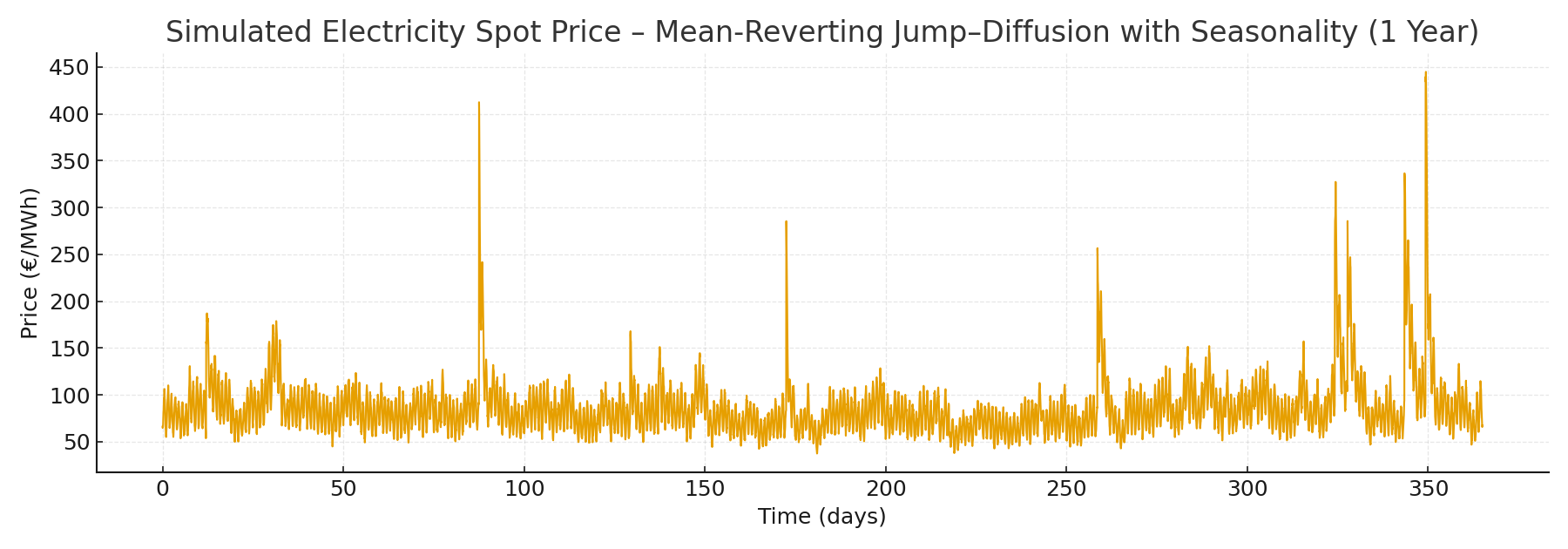
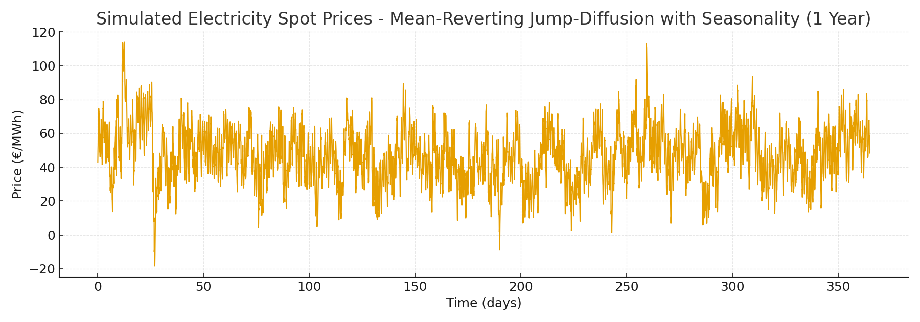
I’ll leave you with two graphical representations of this kind of process (both with a deterministic seasonality layer added but you’ll note the difference between them), and I’ll come back with an article on how you can practically generate such simulations yourself.
References
Clewlow, L., & Strickland, C. (2000). Energy Derivatives: Pricing and Risk Management.
London: Lacima Group.