Analysing The Duration Of Negative Price Spells
March 2026 (2425 Words, 14 Minutes)
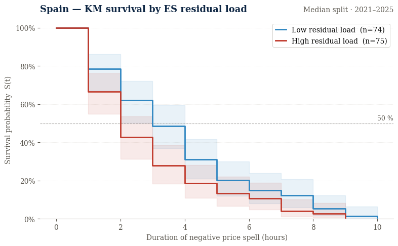
In a previous post, I initiated a discussion (or should I say a monolog ?) about the potential of survival analysis in the energy sector. Inspired by this paper (CITE) focused on price spikes, I started analysing negative price spells in West European day ahead markets from the perspective of their duration rather than their occurence. You can find the complete article here (LINK). Thanks to the Kaplan-Meier estimator and the concept of hazard rate, I uncovered the following stylised facts :
- Spain exhibits the steepest early drop: after ~2 hours, survival is well below 50%.
- France, Belgium and the Netherlands display much higher early survival probabilities — closer to 65–70% after 2 hours. Germany sits in-between.
- The probability of negative price spells lasting longer tends to increase in France with the years, while no clear difference can be spotted in Germany. Germany feels like a system that has already adapted to this phenomenon, while France still appears to be in the middle of that adjustment process.
- In Germany and Spain, as peak RES penetration increases, the survival curves shift upward almost systematically — a strong structural link between renewable oversupply and price persistence.
Kaplan–Meier is great: it tells you the probability that a negative price spell is still ongoing after 1 hour, 2 hours, 6 hours, etc. But it remains a descriptive tool. Today I’d like to go further and uncover why some spells last longer than others, using Cox proportional hazard models.
As in the first article, I’ll use data from the ENTSO-E Transparency platform. I’ll focus on France, Belgium, Germany and Spain — the four countries where the models have shown structurally different results.
This article is organised as follows: the first section gives a solid understanding of the Cox model and describes the procedure I use to build and evaluate it. The other sections are organised by country.
1. The Cox proportional hazard model
The Cox model answers a simple question :
“What factors increase or decrease the probability that a negative price spell ends?”
Instead of modelling duration directly, it focuses on the hazard rate — the probability that the spell ends at this moment, given that it has lasted until now. Think of it as the instantaneous “escape probability” from a negative price regime.
The Cox model assumes that the hazard takes the following form:
\[h(t \mid X) = h_0(t)\, e^{\beta X}\]where:
| Symbol | Meaning |
|---|---|
| \(h(t \mid X)\) | Hazard at time \(t\), given covariates \(X\) |
| \(h_0(t)\) | Baseline hazard — the natural dynamics of the system |
| \(X\) | Explanatory variables (residual load, seasonality, etc.) |
| \(\beta\) | Coefficients estimated by the model |
Let’s decompose this formula. The baseline hazard \(h_0(t)\) represents the probability that a spell ends at time \(t\) when all covariates are neutral. System conditions then multiply this baseline through the exponential term \(e^{\beta X}\).
The exponential has several convenient properties:
- it guarantees the hazard is always positive (\(e^{\beta X} > 0\)),
- effects combine multiplicatively across variables,
- it produces easy-to-interpret hazard ratios: if \(e^{\beta} = 1.5\), a one-unit increase in the variable raises the probability the spell ends by 50%.
🧠 Reading a hazard ratio
The hazard ratio (HR) is the key output of the model:
- HR > 1 → the spell ends faster when this variable increases
- HR < 1 → the spell persists longer when this variable increases
- HR = 1 → the variable has no effect
Example: a German residual load HR of 1.79 means a one-unit increase in residual load raises the probability the spell ends by 79% — demand is absorbing the renewable surplus.
Why semi-parametric?
The Cox model has an elegant property: it is semi-parametric. The effect of the variables is modelled parametrically (we estimate \(\beta\) like in any regression), but the baseline hazard \(h_0(t)\) is left completely unspecified.
This matters because negative electricity price events might end quickly most of the time, but occasionally persist for many hours during oversupply regimes. Rather than forcing this into a specific distribution (exponential, Weibull, log-normal…), the model lets the data speak.
The model focuses entirely on what we care about most: how system conditions modify the probability that the event ends.
2. Variable selection via LASSO
My first challenge was choosing which variables could plausibly influence the duration of negative price events. I relied exclusively on data available through the ENTSO-E API — since day-ahead prices are set the day before delivery, only day-ahead information can be used.
Base variables from ENTSO-E:
- Forecasted load
- Forecasted solar generation
- Forecasted wind generation
- Day-ahead prices
From these, I constructed forecasted residual load (load minus wind and solar) — a proxy for renewable penetration — and lagged price variables (minimum and median price from the previous auction).
Derived residual load indicators (to capture the shape of renewable production throughout the day):
- Median, minimum and maximum residual load during peak hours
- Residual load at 10:00 and 15:00
- Mean residual load during off-peak hours
Calendar variables:
- Weekend and weekday indicators
- Monthly seasonal component (sine and cosine transformations)
Including residual load for neighbouring countries quickly leads to the core problem:
Too many variables. A selection mechanism is needed.
LASSO regularisation
An old reflex led me to LASSO. Instead of maximising the likelihood alone, LASSO maximises a penalised objective:
\[\text{Likelihood} - \lambda \sum |\beta|\]The penalty \(\lambda\) forces some coefficients to shrink toward zero — variables that add little explanatory power simply vanish. The larger \(\lambda\), the simpler the model.
To choose the optimal \(\lambda\), I tested a grid of penalties and selected the one producing the best predictive performance.
3. Evaluating model performance
Two metrics guide model selection. Both are available directly in the lifelines Python package.
📐 Concordance index (C-index)
Measures how well the model ranks durations:
If two spells have different durations, does the model correctly predict which one lasts longer?
- 0.5 → random guess
- 1.0 → perfect ranking
- 0.7–0.8 → already strong for electricity markets, which are inherently noisy
📐 Partial AIC
Balances model fit and model complexity. Lower is better.
AIC rewards models that explain the data well while remaining as parsimonious as possible — penalising unnecessary variables even if they marginally improve fit.
Modelling procedure
The estimation workflow follows five steps:
- Construct candidate explanatory variables
- Apply LASSO regularisation to eliminate redundant features
- Select the optimal penalty using concordance and partial AIC
- Estimate the final Cox model on the selected variables
- Interpret hazard ratios
The goal is not simply to predict duration, but to identify the structural drivers of negative price persistence.
4. Germany: the engine of negative price regimes
The final model for Germany is parsimonious and tells a relatively coherent story.
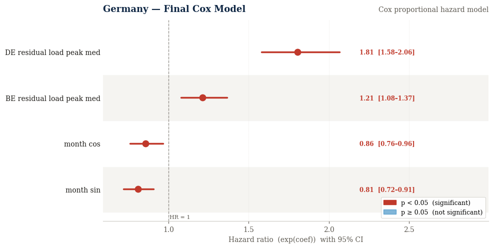
What drives German episodes to end?
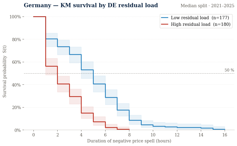
The dominant driver is German residual load during peak hours (HR ≈ 1.79). When demand is stronger relative to renewable generation, the system absorbs excess supply more quickly and negative prices disappear faster. This is consistent with what the Kaplan-Meier analysis already suggested:
Belgian residual load also appears — the only neighbouring country selected — with a smaller HR of about 1.21. Cross-border exchanges help absorb German oversupply, though the effect remains secondary.
Seasonal components (sine and cosine of the month) are both significant, reflecting that certain periods — high renewable output, moderate demand — are structurally more prone to persistent negative prices. Sine and cosine variables aren’t very readable so I reconstrcuted the signal and something interesting appeared :
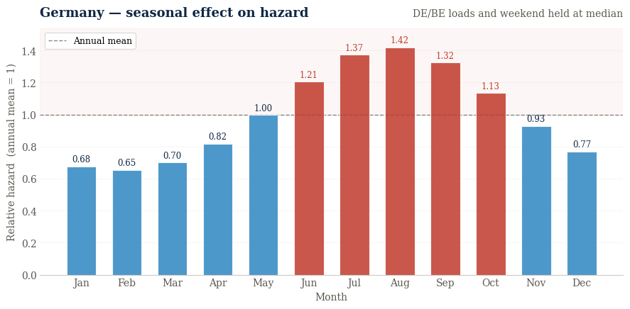
The seasonality effect seems to be the inverse of what we would have expected. Indeed, we have observed over the period longer negative spells during summer but the hazards are higher during this period in the model. It reflects a classic confounding effect. Summer months have lower residual load (high solar output, moderate demand), and low residual load is the dominant driver of persistence. The raw empirical pattern is therefore largely explained by the residual load channel. Once the model strips out that effect, the residual seasonal signal points in the other direction: holding residual load constant, summer is actually associated with faster spell termination.
What could drive this residual seasonal effect? A few mechanisms are plausible:
- Export capacity: cross-border interconnectors are less congested in summer, giving Germany more headroom to export excess supply and resolve negative price episodes faster.
- Demand response: large industrial consumers tend to respond more readily to negative price signals in summer, when their operational constraints differ from winter.
- Nuclear availability in neighbouring markets: high French nuclear output in winter reduces the willingness of neighbouring systems to absorb German oversupply, prolonging episodes in ways that residual load alone does not capture.
These remain interpretations rather than conclusions : properly testing them would require interconnector flow data and cross-border generation schedules that go beyond what ENTSO-E day-ahead forecasts provide.
What doesn’t matter for Germany?
The weekend effect is not significant. Once system balance and seasonality are controlled for, there is no meaningful weekday/weekend difference. Germany’s large industrial base and cross-border flows seem to smooth out intra-week variations.
🔍 Germany — takeaway
The model delivers a coherent economic message: negative price persistence in Germany appears primarily driven by domestic supply-demand balance, with a modest contribution from Belgian system conditions.
That said, the concordance of 0.68 is only reasonable — many short-term operational factors remain unobserved in the ENTSO-E data, which likely limits predictive power.
5. Belgium: a market shaped by its neighbours
The Belgian model reveals a structurally different picture.

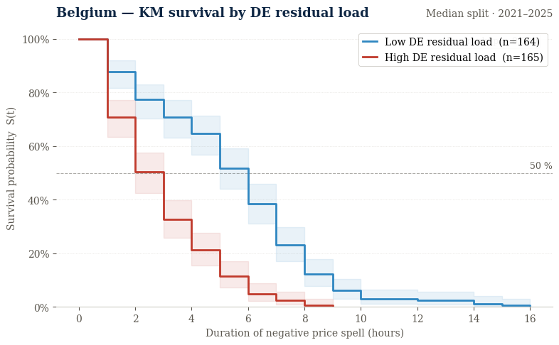
What drives Belgian episodes to end?
German residual load is the dominant factor (HR ≈ 1.63) — more important than Belgium’s own system balance. When Germany absorbs its oversupply, Belgian negative price spells tend to end too. Belgium’s negative price dynamics appear, to a large extent, imported.
Belgian residual load is also significant (HR ≈ 1.47), confirming that local conditions contribute — but remain secondary.
Interestingly, Dutch residual load has a negative effect (HR ≈ 0.79): certain regional configurations prolong Belgian spells. This likely reflects situations where oversupply is shared across interconnected markets, reducing each system’s ability to absorb excess generation.
What doesn’t matter for Belgium?
- Calendar effects (weekday/weekend) — absorbed by stratification
- Price-based variables (lagged day-ahead prices)
- Alternative residual load representations (peak max, off-peak averages, hourly values)
- French residual load — notably absent
This suggests that Belgian negative price persistence is primarily driven by structural system balance, rather than short-term price signals or detailed intra-day patterns.
🔍 Belgium — takeaway
The Belgian model conveys a fairly clear message: negative price persistence is largely driven by regional dynamics, with Germany acting as the main driver and the Netherlands paradoxically prolonging episodes.
The concordance of 0.74 indicates strong predictive performance — the best among the four models — which reinforces the relevance of cross-border system dynamics for Belgium.
6. France: a partially insulated system
The French model is perhaps the most surprising of the four.
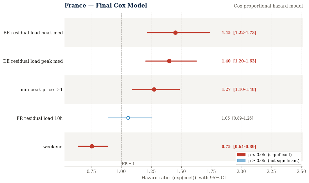
What drives French episodes to end?
Unlike Germany, domestic French residual load does not play a significant role. It was retained by the LASSO procedure — concordance dropped meaningfully without it — but the coefficient itself is small and statistically weak. This is a puzzling result.
One possible interpretation is that French negative price persistence may not be primarily driven by renewable generation in the way it is in Germany. But this conclusion should be treated cautiously: the domestic residual load variable is likely correlated with other selected variables (the weekend indicator and lagged prices in particular), which may explain why its independent effect is hard to isolate.
Cross-border effects dominate instead:
- Belgian residual load: HR ≈ 1.45
- German residual load: HR ≈ 1.41
France seems to behave as part of a broader regional system, where external conditions strongly influence local price dynamics.
Two features unique to France also emerge:
- Lagged prices (minimum peak price from the previous auction, HR ≈ 1.27): France is the only market where price-based variables are retained. This suggests a short-term memory effect — recent auction signals carry information about current system conditions — though the mechanism is not entirely clear.
- Weekend effect (HR ≈ 0.75): negative price spells tend to last longer on weekends, reflecting lower demand and reduced system flexibility. This contrasts with Germany, where the weekend effect vanishes once system balance is controlled for.
What doesn’t matter for France?
- Detailed intra-day residual load representations (hourly values, off-peak averages)
- Seasonal components (month sine/cosine)
🔍 France — takeaway
The French model is harder to interpret than the others. The absence of a significant domestic residual load effect is surprising, and the role of lagged prices is a feature not found elsewhere. Whether this reflects a genuine structural difference in how the French market processes information — or a limitation of the available variables — remains an open question.
The concordance of 0.74 suggests the model has reasonable predictive power despite this ambiguity.
7. Spain: a different negative price dynamic
The Spanish model is structurally different — and clearly less informative than the others.
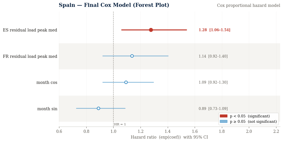
What drives Spanish episodes to end?
The only significant variable is Spanish residual load during peak hours (HR ≈ 1.26). When demand net of renewables rises, the system rebalances and prices recover. The direction is intuitive, but the model cannot say much beyond this single driver.
What doesn’t matter for Spain?
Essentially everything else:
- Cross-border variables (e.g., French residual load)
- Calendar effects (weekend)
- Seasonal patterns (month sine/cosine)
This contrasts with Germany and Belgium, where both domestic and neighbouring conditions play a measurable role.
🔍 Spain — takeaway
The concordance of 0.61 confirms limited predictive power — only marginally better than a random ranking. This is not necessarily a modelling failure: negative prices in Spain are rarer and less persistent over the period studied, and their drivers may involve more localised or complex factors that the ENTSO-E variables cannot capture.
The Cox framework remains valid here, but the signal-to-noise ratio is simply lower.
Conclusion: four markets, four structural stories
The Cox models suggest that negative price persistence is not a single phenomenon — its drivers differ meaningfully across markets.
| Country | Dominant driver | Regional coupling | Unique feature | C-index |
|---|---|---|---|---|
| 🇩🇪 Germany | Domestic residual load (HR 1.79) | Belgium helps (HR 1.21) | Self-contained | 0.68 |
| 🇧🇪 Belgium | German residual load (HR 1.63) | NL prolongs (HR 0.79) | Dynamics largely imported | 0.74 |
| 🇫🇷 France | Regional balance (DE + BE) | Both significant | Price memory + weekend effect | 0.74 |
| 🇪🇸 Spain | Domestic residual load (HR 1.26) | None selected | Structurally harder to explain | 0.61 |
The broader takeaway: negative price risk is about persistence, not just frequency. A histogram tells you how often prices go negative. A Cox model gives you a first approximation of why some markets recover in two hours while others stay negative for six — even if the answer remains partial.