An Intuition For Linear Optimisation And Duality
May 2026 (2698 Words, 15 Minutes)
This note introduces the main ideas behind linear optimisation through a simple electricity dispatch problem. The goal is not to provide a rigorous optimisation course, but to build an intuitive understanding of primal problems, duality, shadow prices and the KKT conditions, and to show how they naturally lead to the economic logic of electricity markets.
We will start with the geometric intuition behind linear problems, then progressively construct the primal problem, the Lagrangian, the dual problem and the KKT conditions before finally discussing where the framework breaks when integer variables are introduced.
Let’s use an electricity dispatch problem as an example. In our imaginary world, there are two power plants available : plant A has a cost of 2€ per MWh produced and a maximum capacity of 100MW and plant B has a cost of 5€ per MWh produced and a capacity of 300MW. Our objective is to minimise the production costs while ensuring the total production equals the demand.
This problem is called linear because every relationship is proportional. For both plants, producing 100MW costs twice as much as producing 50MW. This sounds restrictive: for example we can’t include startup costs because we’ll break the proportionality. However, it’s precisely what makes the problem solvable at scale for a good geometric reason.
This reason is that every constraint in a linear problem draws a straight line (in 2D) or a flat plane (in higher dimensions) across the space of possible decisions. It defines a region of valid solutions : the feasible set which, because all boundaries are straight, always forms a convex polygon. Convexity is the crucial property here:
Because the problem is convex, if two solutions are feasible, then every weighted average of those solutions is also feasible. This geometric structure is what makes linear optimisation tractable and gives dual prices their meaning.
Let’s take our dispatch problem again and try to visualise it geometrically :
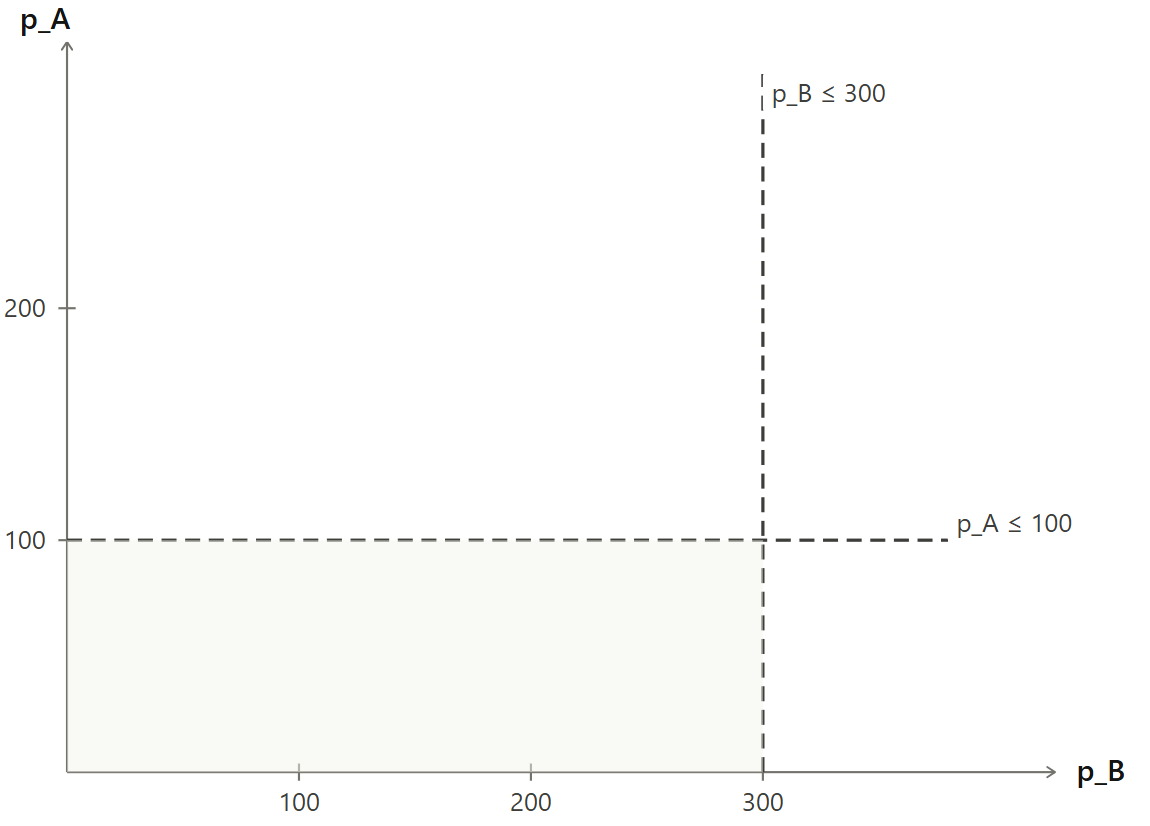
First we draw the capacity constraints for plant A and B :
Second, we add the demand constraint to obtain the feasible region (here we accept overproduction then, unlike in the next sections, our demand constraint is an inequality : \(p_A + p_B \geq 200\))
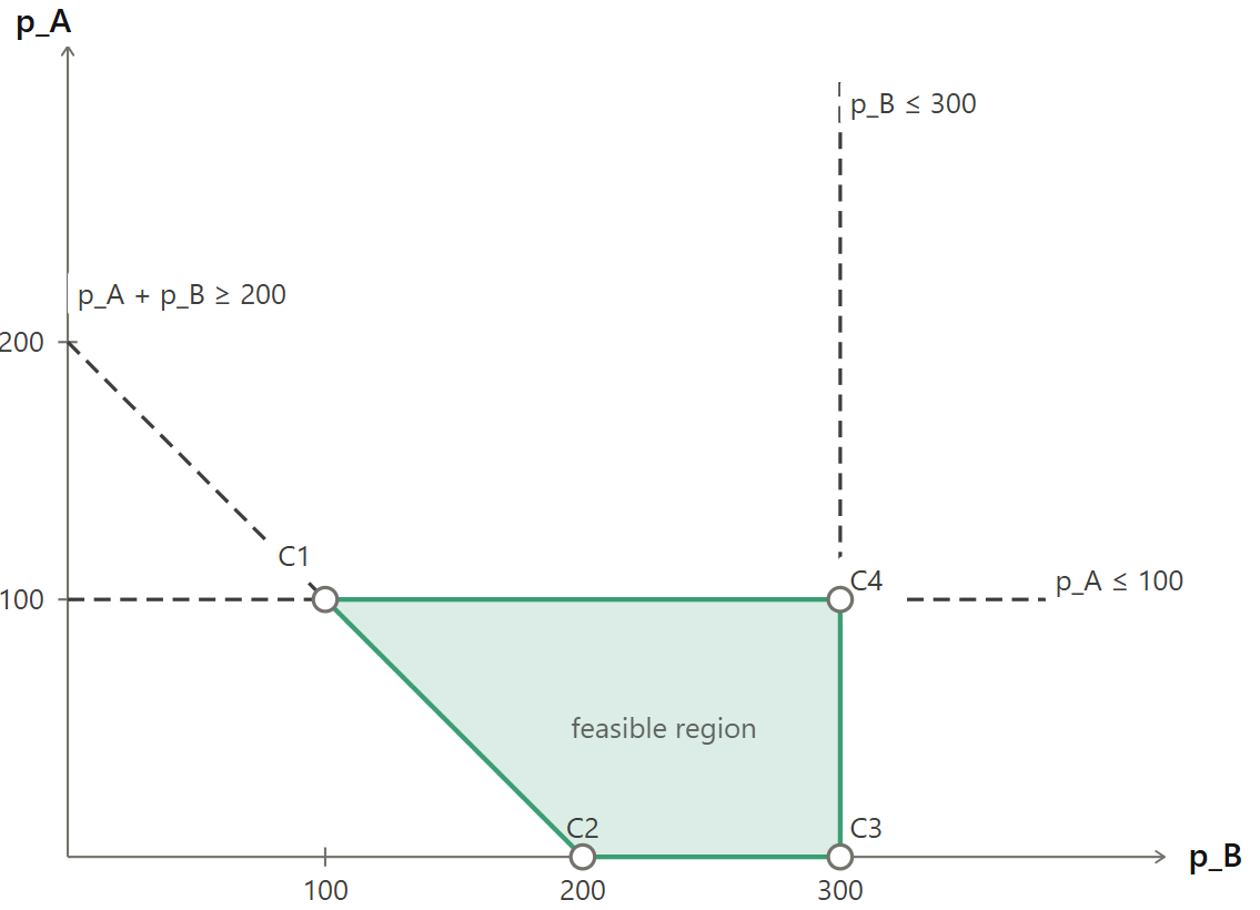
The feasible region is the green area. We have the following critical property :
If a linear problem has a finite optimum, at least one optimum is always located at a corner of the feasible region.
Indeed, an objective function has a direction of improvement “go this way and the cost decreases”. As long as you are in the interior of the feasible region, you can always take a small step in that direction and stay feasible. So the interior is never optimal, you can always do better. When you hit an edge of the region, you’re constrained on one side but can still slide along the edge. As long as the edge is not perpendicular to the direction of improvement, sliding along in the correct direction keeps reducing the cost. You stop only when you hit a corner, because every direction that would further reduce the cost takes you outside the feasible region. You’ve reached the optimum (or at least a candidate optimum).
Using the cost decreasing direction, the cost is evaluated at several corners of the feasible region, finding that point C1 is the optimum (with cost = 700€).
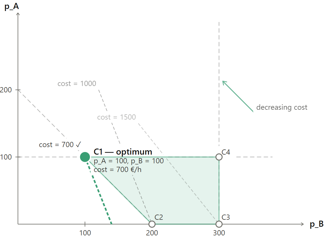
This is roughly how the Simplex algorithm works : it moves from corner to corner along the edges of the feasible region while continuously improving the objective.
Nota Bene: Modern solvers do not necessarily work this way. Many large-scale optimisation problems are instead solved using interior-point methods, which move through the interior of the feasible region rather than along its edges. However, the same geometric structure still underlies the problem : convexity, feasible regions and duality remain the key ingredients.
The primal problem
The problem we introduced can be translated in a mathematical format. Each power plant has a maximum capacity \(PMAX_A = 100MW\) and \(PMAX_B = 300MW\) and their production \(p_A\) and \(p_B\) must remain lower than these capacities (and positive). We then have two first constraints:
\[0 \leq p_A \leq 100\] \[0 \leq p_B \leq 300\]producing one MWh costs \(c_A = 2\)€/MWh using plant A and \(c_B = 5\)€/MWh using plant B. We want to minimise the total cost, that’s the objective function:
\[\min_{p_A, p_B} \quad 2p_A + 5p_B\]Finally, the goal of the dispatch system is to ensure production meets demand (exactly, unlike in our visualisation before where production could be larger than demand), then we must enforce equality between production and demand \(D\). Let’s say the demand at some point is 200MWh :
\[p_A + p_B = 200\]the primal problem can be summarised as
\[\min_{p_A, p_B} \quad 2p_A + 5p_B\] \[\text{s.t.} \quad p_A + p_B = 200 \quad [\lambda]\] \[\quad 0 \leq p_A \leq 100 \quad [\mu_A]\] \[\quad 0 \leq p_B \leq 300 \quad [\mu_B]\]The symbols in brackets are called dual variables (or Lagrange multipliers). They measure how valuable each constraint is at the optimum.
- \(\lambda\) is associated with the demand balance constraint. Economically, it will become the electricity price : the value of supplying one additional MWh of demand.
- \(\mu_A\) and \(\mu_B\) are associated with the capacity constraints. They measure the scarcity value of each plant’s capacity : how much the system would benefit from one additional MW of available capacity.
At this stage they are just unknown variables attached to the constraints. Their economic meaning will emerge naturally once we construct the dual problem.
The Lagrangian
We can now introduce the Lagrangian which is basically a trick to remove the wall caused by the constraints. Instead of forbidding infeasible solutions completely, we temporarily allow them but attach a penalty to each violation. For example, exceeding the capacity of plant A by 1MW introduces an additional term proportional to \(\mu_A\). If \(\mu_A\) is small, violating the constraint is cheap. If it is large, violating the constraint becomes very expensive.
The Lagrangian of our dispatch problem is :
\[\mathcal{L} = \underbrace{2p_A + 5p_B}_{\text{original cost}} + \underbrace{\mu_A(p_A - 100)}_{\text{penalty for exceeding A's capacity}} + \underbrace{\mu_B(p_B - 300)}_{\text{penalty for exceeding B's capacity}} - \underbrace{\lambda(p_A + p_B - 200)}_{\text{penalty for missing demand}}\]Now suppose that :
- the primal variables satisfy the original constraints,
- and the multipliers satisfy \(\mu_A, \mu_B \geq 0\).
Then the additional terms are always non-positive :
- if \(p_A \leq 100\) then \(\mu_A(p_A - 100) \leq 0\),
- if \(p_B \leq 300\) then \(\mu_B(p_B - 300) \leq 0\),
- and if demand is exactly met then \(p_A + p_B - 200 = 0\).
This gives the key property :
For feasible primal solutions, the Lagrangian is always less than or equal to the primal cost.
So if we minimise the Lagrangian over \(p_A\) and \(p_B\), the result can never exceed the true optimal value of the primal problem. The Lagrangian therefore provides a lower bound on the primal optimum.
We can rearrange the Lagrangian :
\[\mathcal{L} = \underbrace{(2 - \lambda + \mu_A)}_{\text{coefficient of } p_A} p_A + \underbrace{(5 - \lambda + \mu_B)}_{\text{coefficient of } p_B} p_B + 200\lambda - 100\mu_A - 300\mu_B\]We note \(g(\lambda, \mu_A, \mu_B) = \min_{p_A, p_B \geq 0} \mathcal{L}(p_A, p_B, \lambda, \mu_A, \mu_B)\)
The minimum over \(p_A\) and \(p_B\) is:
- \(-\infty\) if \((2 - \lambda + \mu_A) < 0\) (you’d push \(p_A\) to \(+\infty\))
- \(-\infty\) if \((5 - \lambda + \mu_B) < 0\) (same reason)
- \(200\lambda - 100\mu_A - 300\mu_B\) if \((2 - \lambda + \mu_A) \geq 0\) and \((5 - \lambda + \mu_B) \geq 0\)
So g is only useful in the third case when both constraints over \(\mu_A\) and \(\mu_B\) are satisfied.
The dual problem
We know that \(g()\) is a lower bound of the primal and we would like to find the highest possible lower-bound. That’s when the dual problem emerges :
\[\max_{\lambda, \mu_A, \mu_B} \quad 200\lambda - 100\mu_A - 300\mu_B\] \[\text{s.t.} \quad \lambda - \mu_A \leq 2 \quad \text{(plant A)}\] \[\quad \lambda - \mu_B \leq 5 \quad \text{(plant B)}\] \[\quad \mu_A, \mu_B \geq 0\]Economically, the dual problem is asking : find the prices that maximise the total value of the system’s resources, subject to the constraint that no plan is over rewarded. The variables are :
- \(\lambda\) the electricity price
- \(\mu_A\) and \(\mu_B\) the scarcity values of each plant’s capacity (the extra value an additional MW of capacity would bring to the system).
The great property of linear optimisation is strong duality.
\[\underbrace{2 \times 100 + 5 \times 100}_{\text{primal: total cost}} = \underbrace{200 \times 5 - 100 \times 3 - 300 \times 0}_{\text{dual: total value}} = 700 \text{ €/h}\]Strong duality means that when they are linear problems, the primal and the dual problems give exactly the same number.
This equality is not a coincidence. It says that in a competitive market, the minimum cost of producing electricity equals the total revenue generators earn selling at the market price, minus the scarcity paid to capacity owners.
| Dual variable | Value | Meaning |
|---|---|---|
| \(\lambda\) | \(5\) €/MWh | Plant B sets the price — it’s the marginal unit |
| \(\mu_A\) | \(3\) €/MWh | Plant A earns 3 €/MWh above its cost because it’s capacity-constrained |
| \(\mu_B\) | \(0\) | Plant B has spare capacity — it’s not scarce |
Plant A produces at 2€/MWh but sells at 5€/MWh. the difference (3€/MWh) is its infra-marginal rent. it exists not because plant A is doing anything special but because its capacity is scarce. If you built more of plant A, the rent would shrink. if you built enough to fully replace plant B, the rent would disappear and the price would fall to 2€/MWh.
This is the economic mechanism behind the merit order effect of renewables for example : adding zero-cost solar capacity is equivalent to adding more cheap plant. It pushes more expensive plants off the margin, destroys their role as price setter and collapses both the price and the infra-marginal rents of all other generators simultaneously.
The KKT conditions
We now have all the pieces : the primal dispatch problem, the dual price system, the Lagrangian that connects them. The KKT conditions are the three rules that any optimal solution must satisfy simultaneously. They are properties that emerge automatically at the optimum, not additional constraints.
Condition 1 — Stationarity : the price is pinned by the marginal plant
At the optimum, the Lagrangian cannot be improved by nudging any production variable. Mathematically this means the derivative of the Lagrangian with respect to each \(p_g\) is zero. For plant A this gives :
\[\lambda = c_A + \mu_A\]For plant B :
\[\lambda = c_B + \mu_B\]That means : the electricity price equals the marginal cost of each plant plus its scarcity rent.
For plant B, which is not capacity-constrained, \(\mu_B = 0\) and the condition becomes \(\lambda = c_B = 5\). The price is exactly plant B’s marginal cost, and that makes sense because plant B is the marginal unit (the last one dispatched which therefore sets the price).
For plant A, which is at full capacity, \(\mu_A = 3\) and the condition gives \(\lambda = 2 + 3 = 5\). Plant A’s cost plus its scarcity rent equals the market price. The scarcity rent is exactly the gap between what plant A costs and what the market pays : it’s the infra-marginal rent that plant A earns by being cheaper than the price-setter.
This condition is the mathematical expression of the merit order : the price is always set by the marginal unit, and every cheaper unit earns a rent equal to the difference between the price and its own cost.
Condition 2 — Complementary slackness : scarcity and spare capacity cannot coexist
For each capacity constraint, the following must hold:
\[\mu_g \cdot (\overline{P}_g - p_g) = 0\]This says : either the plant is at full capacity (\(\overline{P}_g - p_g = 0\)) or its scarcity rent is zero (\(\mu_g = 0\)). Both cannot be non-zero simultaneously.
The economic logic is immediate. If a plant has spare capacity (is producing below its maximum) then one more MW from that plant costs nothing extra to unlock. Its capacity is not the binding constraint. It has no scarcity value, so \(\mu_g = 0\).
If a plant has a positive scarcity rent (its capacity is genuinely valuable) then it must be running at its limit. If it weren’t, you could produce more from it and save money, which contradicts optimality.
In our example :
- Plant A : running at 100 MW \(= \overline{P}_A\), so \(\mu_A = 3 > 0\) ✓
- Plant B : running at 100 MW \(< \overline{P}_B = 300\), so \(\mu_B = 0\) ✓
This condition is what connects the primal dispatch to the dual prices. It tells you exactly which constraints are “active” and which are slack. An active constraint has a positive dual variable. A slack constraint has a zero dual variable. This is how you read the economics of the whole system at a glance.
Condition 3 — Primal feasibility : the solution must be physically valid
The optimal solution must respect all the original constraints :
\[p_A + p_B = 200 \quad \text{(demand met)}\] \[0 \leq p_A \leq 100, \quad 0 \leq p_B \leq 300 \quad \text{(capacity limits)}\]This may sound obvious but it matters formally because the Lagrangian approach technically allows infeasible solutions during the search process. The KKT conditions require that at the optimum, you are back inside the feasible set.
The three conditions together reproduce the merit order
Primal feasibility says demand is met. Stationarity says the price is set by the marginal unit. Complementary slackness says cheap units run at full capacity and earn a scarcity rent and expensive units stay idle and earn nothing. Only the marginal unit sits in between, producing at whatever level is needed to balance supply and demand, with zero scarcity rent because it has spare capacity.
This is precisely the simplified merit order which appears as the unique solution that satisfies all three KKT conditions simultaneously. Any other dispatch would violate at least one of them.
How solvers use these conditions in practice
The KKT conditions play a double role in practice.
During the solve, they serve as the stopping criterion. At each iteration, the solver checks whether the current solution satisfies the KKT conditions to within a numerical tolerance (typically \(10^{-7}\)). As long as any condition is violated, the algorithm keeps iterating. The moment all three are satisfied within tolerance, the solver stops and declares the solution optimal. This is why you see parameters like primal_feasibility_tolerance and dual_feasibility_tolerance in HiGHS.
After the solve, they serve as a validation tool. When your model produces an unexpected price the KKT conditions give you a systematic diagnostic protocol. You find the plant satisfying \(\lambda = c_g\) (the marginal unit), verify that all cheaper plants satisfy \(\mu_g > 0\) and are running at capacity, and verify that all more expensive plants satisfy \(p_g = 0\). If any of these checks fail, there is a bug in your formulation. The KKT conditions turn a black-box output into an auditable economic narrative.
Bonus section — When the framework breaks : adding integer variables
Everything we have built so far relies on one assumption: all decision variables are continuous. Production can be set to any value between 0 and \(\overline{P}_g\). This is what makes the problem linear, the feasible set convex, and the dual prices meaningful.
This assumption breaks the moment you introduce non-linearities such as startup costs. A startup cost is only paid if a plant actually starts which requires a variable that captures the on/off decision : \(u_g \in \{0, 1\}\). One binary variable is enough to destroy the entire LP structure.
Indeed, binary variables turn the feasible set from a convex polygon into a collection of discrete points. Simplex no longer has edges to slide along. Strong duality no longer holds (the primal and dual optimal values are no longer guaranteed to be equal). The KKT conditions do not apply.
The practical fix used in power system modelling is a two-step procedure. First, solve the MILP to find the optimal commitment — which plants are on or off at each hour. Then fix those binary decisions and re-solve the resulting LP, where all remaining variables are continuous. This resulting LP is convex, its dual is well-defined, and its shadow prices are interpretable as market prices, conditional on the commitment found in step one.
The economic consequence of this two-step approach is subtle but important. Some plants that were committed in the MILP may find themselves operating at a loss at the LP market price : they were worth committing for system reasons, but the price doesn’t cover their startup cost. In real markets, this could be resolved through uplift payments : out-of-market side payments that compensate committed units for losses they incur at the market price. The clean merit order world of the LP is an approximation.